
Spark’s Coalesce vs Repartition vs Repartition-by-Range – My Experience with them
If you’ve spent any time tuning Spark jobs, you’ve run into the classic question: do I call `coalesce()`, `repartition()`, or `repartitionByRange()`? All three change how your data is partitioned across the cluster, but they behave very differently under the hood — and choosing the wrong one is one of the easiest ways to either tank performance or quietly produce skewed output.
This post walks through each one visually, explains the shuffle that sits underneath two of them, and ends with a decision flow and real examples from a production data pipeline I’ve been working on — the Data Platform — where the right choice between these three made the difference between a job that finished in minutes and one that crashed the executor.
A quick mental model: what is a partition?
Before we compare the three, let’s anchor on what a partition actually is.
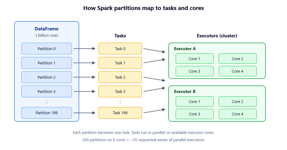
When Spark reads data, it splits it into chunks called partitions. Each partition is a unit of parallel work — one task per partition, running on one core somewhere on the cluster.
Too few partitions and you underutilize the cluster. Too many and you drown in scheduling overhead. The three functions below are how you reshape that partitioning when the defaults aren’t right.
First, the elephant in the room: what is a shuffle?
You can’t talk about repartition or repartitionByRange without understanding shuffles, because that’s what makes them expensive. A shuffle is what happens whenever Spark has to physically move data between executors so that related rows can sit together in the same partition.
A shuffle gets triggered by any wide transformation — groupBy, join, distinct, orderBy, and yes, repartition and repartitionByRange. Narrow transformations like filter, map, and select don’t need it because each output partition depends only on a single input partition.
Here’s what’s actually happening when a shuffle runs:
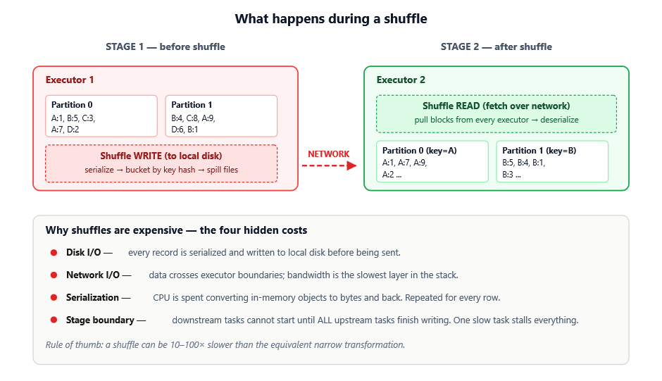
Notice that the cost isn’t one thing — it’s four costs stacking on top of each other:
1. Disk I/O — every record is serialized and written to local disk first. Even before any network transfer, you’re paying for sequential disk writes on every executor.
2. Network I/O — data has to physically move between machines. Network bandwidth is the slowest layer of the entire stack, often 10–100× slower than memory access.
3. Serialization / deserialization — JVM objects can’t be sent over a wire as-is. They have to be converted to bytes on the sender and reconstructed on the receiver, burning CPU on both ends.
4. Stage boundary stall — this one is the most overlooked. Downstream tasks cannot start until all upstream tasks finish writing their shuffle output. A single slow task blocks everything behind it.
This is why in the Data platform project we treat shuffles like an audit checkpoint — every time one appears in the physical plan, we ask: is this shuffle earning its keep? If a stage can be restructured to avoid one, that’s almost always a worthwhile rewrite. And when a shuffle is unavoidable, picking the right partitioning function is how you make sure it pays for itself.
With that out of the way, let’s look at the three operations.
1. coalesce(n) — the cheap shrinker
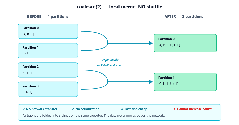
coalesce reduces the number of partitions without a full shuffle. It works by merging existing partitions on the same executor wherever possible.
What you need to know
- It only goes down. coalesce can reduce partitions but cannot increase them. Calling coalesce(1000) on a 10-partition DataFrame just gives you 10 partitions back.
- No shuffle. Data doesn’t move across the network — Spark just stops processing some partitions and folds them into others. That’s why it’s fast.
- Skew is possible. Since it merges whatever’s nearby rather than redistributing globally, you can end up with uneven partitions.
- It can hurt upstream parallelism. This is the subtle gotcha. If you have a heavy transformation followed by coalesce(1), Spark may execute the entire upstream pipeline with just one task, because partitioning propagates backward through narrow dependencies.
How we use it in our Data Platform
In Data platform, we use coalesce in two distinct places, for two different reasons:
1. Producing a single output file per chunk. The matching pipeline writes a CSV of matched record pairs to S3. Downstream consumers expect one file per chunk, not Spark’s default directory of part-00000, part-00001, etc. So at the very end, after all the matching logic is done:
df.write.mode("overwrite").option('header','false').csv(s3_data_output_path_root_with_chunk)
    # then merged via copyMerge into a single final file
We don’t coalesce(1) directly here — we let Spark write multiple files and merge them externally — precisely because coalesce(1) before the write would have collapsed the entire match computation to a single task and killed throughput.
2. Writing a single Parquet file in the preprocessing step. When the preprocessing job produces a processed base file that the matching job needs to read by a known path:
    df.coalesce(1).write.parquet(output_path)
    # then move the single part-file to a deterministic location
Here coalesce(1) is safe because preprocessing is already cheap and the input is small enough that one task can handle it.
The lesson: coalesce(1) is great for producing one file, but only when the upstream work isn’t heavy. If it is, write multiple files and merge externally.
2. repartition(n) or repartition(n, col) — the full reshuffler
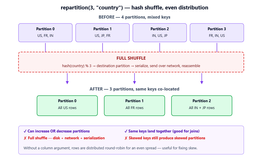
repartition performs a full shuffle, redistributing data evenly (or by a hash of a chosen column) across n partitions.
What you need to know
- Goes up or down. You can ask for any partition count, including more than you started with.
- Full shuffle = expensive. Everything from the shuffle section above applies. Plan for it.
- Even distribution by default. Without a column argument, rows are spread round-robin — great for fixing skew.
- Hash partitioning by column. When you pass a column, rows with the same key land in the same partition. Useful before a join or groupBy to co-locate data and avoid a shuffle later.
- Collisions are possible. Hash partitioning means all rows with the same key go together, but multiple keys can share a partition. If one key dominates the data, you’ll still get skew.
How we use it in our Data Platform
Data platform hit a memory wall when running the Caverphone2 phonetic matching across millions of records on EMR Serverless — a SocketException thrown by the JVM, caused by a Python worker getting killed under memory pressure. Part of the fix was controlling parallelism explicitly with repartition:
  # Limit concurrent tasks to fit within the 4 GB executor heap
    df = df.repartition(4)   # cap simultaneous workers
    # ... heavy transformation runs ...
    df.coalesce(2).write.parquet(...)   # then narrow down for the write
The repartition(4) ensures we have exactly four partitions feeding the heavy Caverphone2 step, so we never get more than four Python workers competing for memory at the same time. The coalesce(2) after it shrinks the writer count without re-shuffling. Combined with switching to a pandas_udf, this was what stopped the executor from crashing.
We also use repartition before our full-outer joins of the three match groups:
df = df1.join(df2, ['index_col', 'index_col'], how="fullouter")
Pre-partitioning on the join keys (when spark.sql.adaptive.enabled doesn’t already handle it) cuts the shuffle volume during the join itself.
3. repartitionByRange(n, col) — the sorted distributor
repartitionByRange also performs a full shuffle, but instead of hashing the key, it partitions by ordered ranges of the key. Spark samples the data to estimate boundaries, then assigns rows to partitions based on where they fall in the sorted order.
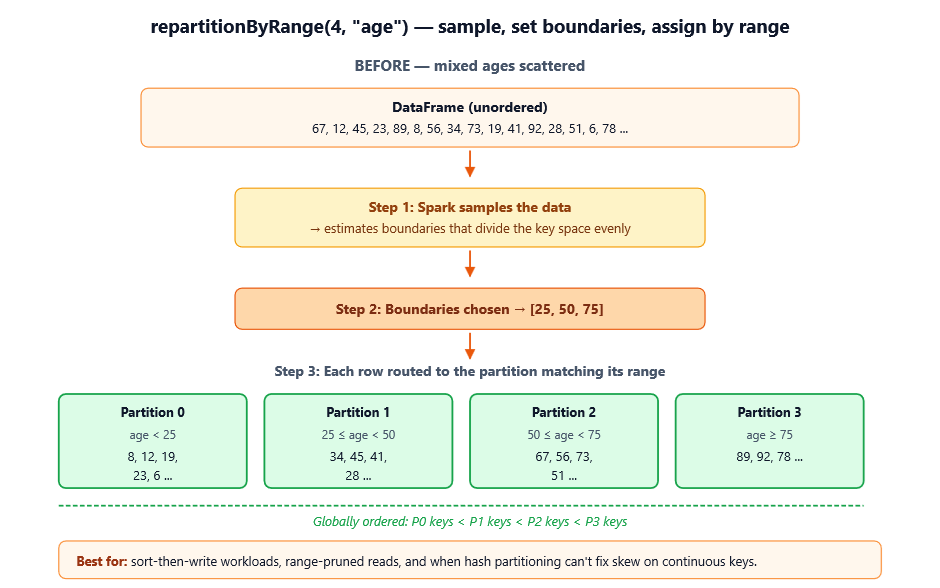
What you need to know
- Ordered partitions. Partition 0 contains the smallest keys, partition n-1 the largest. Within a partition, data isn’t necessarily sorted, but across partitions, the ordering holds.
- Sample-based. Spark takes a sample to estimate boundaries, so distribution is approximate but typically very even — even when the data is skewed.
- Best on continuous or naturally ordered keys. Numeric columns, timestamps, alphabetized strings.
- Bad on categorical / low-cardinality keys. If your column has only a handful of distinct values, range partitioning collapses to something close to a single partition per value.
Where it would fit in our platform (and where it wouldn’t)
Honestly, repartitionByRange is the one we use least in our platform— our match keys are categorical (encoded surrogate keys), so hashing works better than ranging. But it’s the right tool the moment we move to time-partitioned output, e.g. when archiving matched pairs by match_date for downstream BI consumption:
    results.repartitionByRange(50, "col") \
           .write.partitionBy("col") \
           .parquet("s3://dms-archive/matches/")
This ensures each output file contains a contiguous date range, so analytical queries with WHERE match_date BETWEEN ‘…’ AND ‘…’ can prune most files at the metadata level without ever opening them. Hash partitioning would scatter the dates and break that pruning.
Side-by-side comparison
| Aspect | `coalesce(n)` | `repartition(n[, col])` | `repartitionByRange(n, col)` |
| Shuffle? | No | Yes (full) | Yes (full) |
| Can increase partitions? | No | Yes | Yes |
| Can decrease partitions? | Yes | Yes | Yes |
| Distribution strategy | Local merge | Round-robin or hash | Sampled ranges |
| Output ordering | Preserved within merged partitions | None | Globally ordered by key |
| Risk of skew | Possible (merges whatever’s there) | Possible on skewed keys | Low (sampling balances) |
| Cost | Cheap | Expensive | Expensive + sampling |
| Typical use | Shrink for output | Even out / pre-shuffle for join | Pre-sort, range pruning |
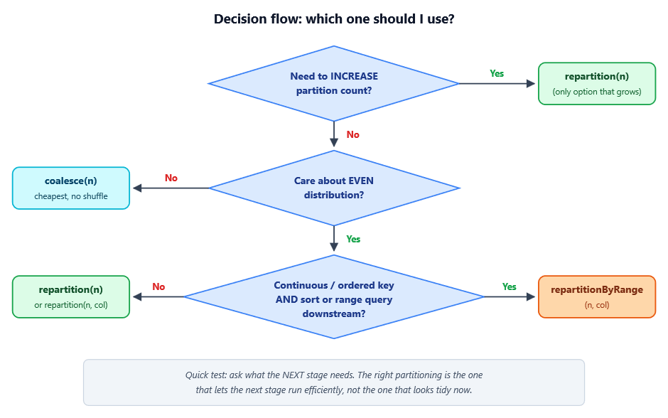
A decision flow
When you find yourself reaching for one of these, walk through this:
Three traps to watch for
1. `coalesce(1)` killing your job. Writing to a single file feels tidy, but if it comes after a heavy transformation, Spark may collapse the entire upstream pipeline to one task. We learned this firsthand in our platform— our first attempt at coalesce(1) before the matching step caused the whole pipeline to serialize through a single executor. The fix was to write many files and merge externally with a copyMerge-style helper.
2. `repartition` on a skewed column. Hashing doesn’t fix skew if 80% of your rows share the same key. They all still land in the same partition. Either pre-salt the key, or use repartitionByRange if the column is continuous. Better yet, turn on spark.sql.adaptive.skewJoin.enabled so AQE handles it at runtime.
3. `repartitionByRange` on low-cardinality data. If your “key” has 5 distinct values and you ask for 200 partitions, you’ll get 5 non-empty partitions and 195 empty ones. Range partitioning needs spread.
Wrapping up
The three operations live on a spectrum of cost and control:
- `coalesce` is the lightweight tool for shrinking partitions when you don’t care about evenness.
- `repartition` is the workhorse — full shuffle, even distribution, or hash-based co-location.
- `repartitionByRange` is the specialist — when you need ordering or are about to sort.
In the Data Platform, applying these correctly — repartition(4) to bound memory during Caverphone2 matching, coalesce(1) for single-file preprocessing outputs, and external merging instead of coalesce(1) for the heavy match step — turned a job that was crashing executors with SocketException into one that runs cleanly on a 4 GB heap. None of these are exotic optimizations. They’re just the difference between calling the right function at the right point in the pipeline.
The best Spark engineers I know don’t memorize which one to use; they reason about what their downstream stage needs and pick the partitioning that sets that stage up to win. Coalesce when you’re done. Repartition when you need balance or co-location. Range-partition when order matters.
Next time you’re staring at a slow stage in the Spark UI, ask yourself which one of these the job is really asking for — chances are, you’ll find your answer.